Percolation

Introduction

Percolation theory is a fundamental concept in statistical physics and mathematics that describes the behavior of connected clusters in a random graph. It is a model for understanding how a network behaves when nodes or links are added, leading to a phase transition from a state of disconnected clusters to a state where a large, connected cluster spans the system. This transition occurs at a critical threshold, known as the percolation threshold. The theory has applications in various fields, including material science, epidemiology, and network theory.

Why is Percolation Important? Useful Applications

Percolation theory is important because it provides insights into the behavior of complex systems and phase transitions. Here are some key applications:

Material Science: Percolation theory helps in understanding the properties of composite materials, such as conductivity and strength. For example, the electrical conductivity of a composite material can change dramatically when the concentration of conductive filler reaches the percolation threshold
Epidemiology: In the study of disease spread, percolation models can predict the outbreak and spread of epidemics. The percolation threshold can represent the critical point at which a disease becomes widespread in a population
Network Theory: Percolation theory is used to study the robustness and connectivity of networks, such as the internet or social networks. It helps in understanding how networks can be disrupted and how they can be made more resilient
Geophysics: In oil recovery, percolation theory models the flow of fluids through porous rocks, helping to optimize extraction processes
Forest Fires: Percolation models can simulate the spread of forest fires, helping in the development of strategies for fire prevention and control

Mathematical and Physics Theory

Percolation theory can be studied using site percolation or bond percolation models. In site percolation, each site (or node) on a lattice is either occupied with probability $ p $ or empty with probability $ 1 - p $. In bond percolation, each bond (or edge) between sites is open with probability $ p $ or closed with probability $ 1 - p $.

Step-by-Step Explanation:

Define the Lattice: Consider a 2D square lattice or a 3D cubic lattice. For simplicity, let’s use a 2D square lattice.
Assign Probabilities: For each site (or bond), assign a probability $ p $ that it is occupied (or open).
Cluster Formation: Identify clusters of connected sites (or bonds). Two sites are in the same cluster if there is a path of occupied sites (or open bonds) connecting them.
Critical Threshold $ p_c $: Determine the critical probability $ p_c $ at which an infinite cluster first appears. For a 2D square lattice, it has been rigorously shown that $ p_c \approx 0.5927 $.
Mathematical Formulation: The percolation probability $ P(p) $ is the probability that a given site belongs to the infinite cluster. Near the critical threshold, this follows a power-law behavior: $$ P(p) \sim (p - p_c)^\beta $$ where $ \beta $ is a critical exponent and equal to $\frac{5}{36}$ for 2D squared lattice.
Correlation Length $ \xi $: The average size of finite clusters below $ p_c $ is characterized by the correlation length $ \xi $, which diverges as: $$ \xi \sim |p - p_c|^{-\nu} $$ where $ \nu $ is another critical exponent
Conductivity and Other Properties: In practical applications, properties like electrical conductivity in materials can be modeled by considering the effective medium theory or numerical simulations to calculate the likelihood of percolation and the size of clusters.

By analyzing these steps, percolation theory provides a comprehensive understanding of how macroscopic properties emerge from microscopic randomness, revealing universal behaviors that transcend specific systems.

Python Simulation Code

Here is a simple example of a site percolation simulation on a square lattice in Python:

# -*- coding: utf-8 -*-
"""
Created on Wed Jun 19 07:15:50 2024

@author: stefa
"""

import numpy as np
import matplotlib.pyplot as plt
import scipy.ndimage

def generate_lattice(n, p):
    """Generate an n x n lattice with site vacancy probability p."""
    return np.random.rand(n, n) < p

def percolates(lattice):
    """Check if the lattice percolates."""
    intersection = get_intersection(lattice)
    return intersection.size > 1

def get_intersection(lattice):
    """Check if the bottom labels or top labels have more than 1 value equal    """
    labeled_lattice, num_features = scipy.ndimage.label(lattice)
    top_labels = np.unique(labeled_lattice[0, :])
    bottom_labels = np.unique(labeled_lattice[-1, :])
    print(top_labels, bottom_labels, np.intersect1d(top_labels, bottom_labels).size)
    return np.intersect1d(top_labels, bottom_labels)

def plot_lattice(lattice):
    """Plot the lattice."""
    plt.imshow(lattice, cmap='binary')
    plt.show()
  
def lattice_to_image(lattice):
    """Convert the lattice in an RGB image (even if will be black and white)"""
    r_ch = np.where(lattice, 0, 255)
    g_ch = np.where(lattice, 0, 255)
    b_ch = np.where(lattice, 0, 255)
  
    image = np.concatenate((
        np.expand_dims(r_ch, axis=2),
        np.expand_dims(g_ch, axis=2),
        np.expand_dims(b_ch, axis=2),
        ), axis=2)
  
    return image

def get_path(lattice):
    intersection = get_intersection(lattice)
    labeled_lattice, num_features = scipy.ndimage.label(lattice)
    print(intersection)
    return labeled_lattice == intersection[1]

def add_path_img(image, path):
    blank_image = np.zeros(image.shape)
    # set the red channel to 255-> get a red percolation path
    image[path, 0] = 255
    image[path, 1] = 20
    return image
  


# Parameters
n = 100  # Lattice size
p_values = [0.2, 0.3, 0.4, 0.5, 0.58, 0.6]  # Site vacancy probabilities

# Create a figure with subplots
fig, axs = plt.subplots(2, 3, figsize=(15, 8))
axs = axs.flatten()


# Plot lattices for different p values
for i, p in enumerate(p_values):
    lattice = generate_lattice(n, p)
    lattice_img = lattice_to_image(lattice)
    if percolates(lattice):
        axs[i].set_title(f"p = {p} (Percolates)")
        path = get_path(lattice)
        lattice_img = add_path_img(lattice_img, path)
    else:
        axs[i].set_title(f"p = {p} (Does not percolate)")
    axs[i].imshow(lattice_img)
    axs[i].axis('off')

# Adjust spacing between subplots
plt.subplots_adjust(wspace=0.1, hspace=0.1)


# Show the plot
plt.show()

This code generates a square lattice of size n with site vacancy probability p, checks if the lattice percolates (i.e., if there is a connected path from the top to the bottom), and plots the lattice.

In further version, also a connected path from left to right can be considered.

Results

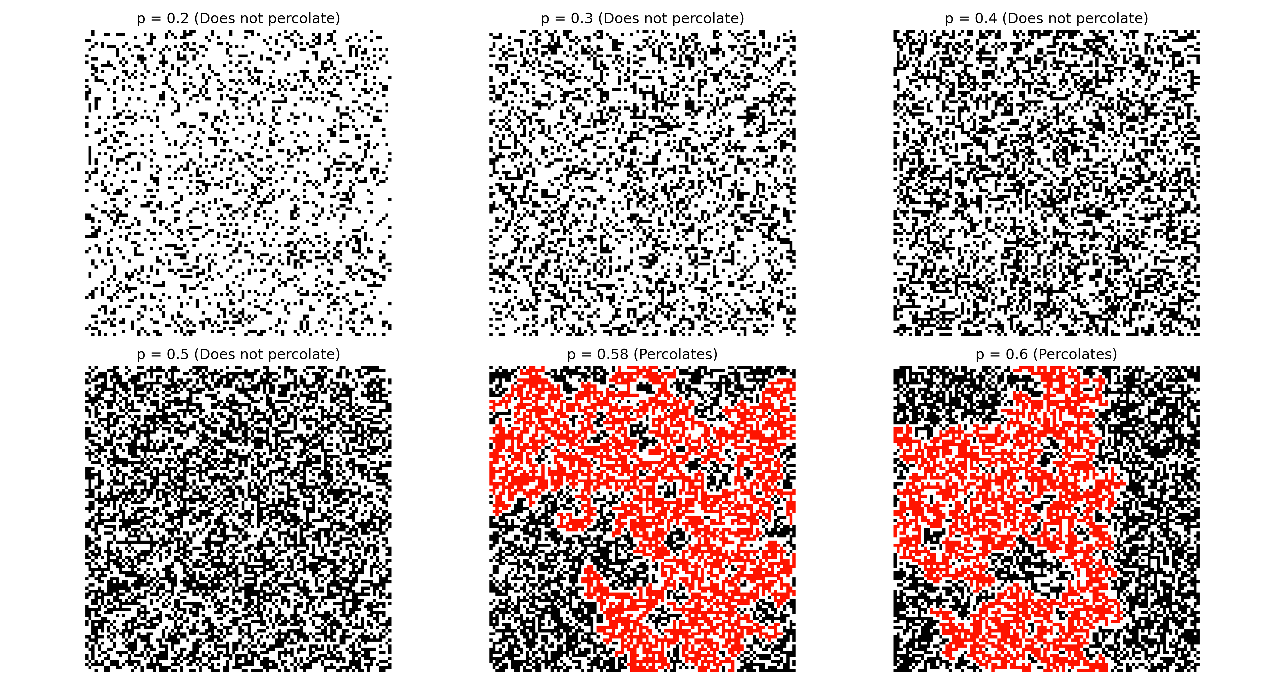
Conclusion

The previous plot shows that with p>0.58 a percolation path starts to be observed. However, this is so not alwasy happening for stochastical reasons. Hence that plot is the result of several iteration to find the most interesting plot. With p>0.60 percolation happens more than 90% of the time. In general, this confirms the numerical value of $p_c$ that can be found in literature of 0.5927

In further articles we will explore some python libraries to develop a more advanced and practical example.

Stefano Giannini