Gemma-2 + RAG + LlamaIndex + VectorDB

Open in:

1. Introduction

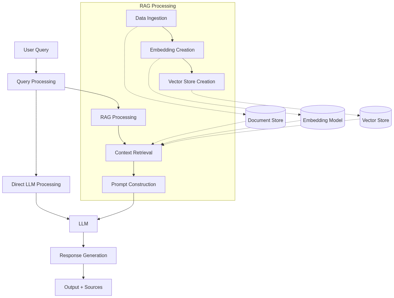
Retrieval-Augmented Generation (RAG) is an advanced AI technique that enhances large language models (LLMs) with the ability to access and utilize external knowledge. This guide will walk you through a practical implementation of RAG using Python and various libraries, explaining each component in detail.

2. Setup and Import

%pip install transformers accelerate bitsandbytes flash-attn faiss-cpu llama-index -Uq
%pip install llama-index-embeddings-huggingface -q
%pip install llama-index-llms-huggingface -q
%pip install llama-index-embeddings-instructor llama-index-vector-stores-faiss -q

import contextlib
import os
import torch

device = torch.device("cuda" if torch.cuda.is_available() else "cpu")
device

device(type=‘cuda’)

from huggingface_hub import login
from kaggle_secrets import UserSecretsClient # use this only in Kaggle, for other platform set your huggingface API secret key in an another way

# Get Secret HuggingFace token (only in Kaggle)
user_secrets = UserSecretsClient()
secret_value = user_secrets.get_secret("huggingface_api")

login(token=secret_value)

3. Model and VectorDB imports

This section imports various components from llama_index for document processing, indexing, and querying.
It sets up FAISS (Facebook AI Similarity Search) for efficient similarity search in high-dimensional spaces.

from transformers import AutoTokenizer, AutoModelForCausalLM, BitsAndBytesConfig
from IPython.display import Markdown, display

from llama_index.core import SimpleDirectoryReader, VectorStoreIndex, ServiceContext
from llama_index.embeddings.huggingface import HuggingFaceEmbedding
from llama_index.llms.huggingface import HuggingFaceLLM
from llama_index.core import set_global_tokenizer

from llama_index.core import (
    SimpleDirectoryReader,
    load_index_from_storage,
    VectorStoreIndex,
    StorageContext,
)

from llama_index.vector_stores.faiss import FaissVectorStore
import faiss

4. Data Loading

Use SimpleDirectoryReader from llama_index.

#  Load the PDF
documents = SimpleDirectoryReader('/kaggle/input/superconductivity-lectures/').load_data()

5. Load Embedding Model

It uses the “sentence-transformers/all-MiniLM-L6-v2” model to create vector representations of text.
This model is known for its efficiency in creating semantic embeddings.

# Load embedding model
embed_model = HuggingFaceEmbedding(model_name="sentence-transformers/all-MiniLM-L6-v2")

6. Language Model Setup and Loading

It uses the “google/gemma-2-9b-it” model, a powerful instruction-tuned language model.
It configures 8-bit quantization to reduce memory usage
The tokenizer is set globally for consistency.
The model is configured with specific generation parameters and quantization for efficiency.

from transformers import AutoTokenizer, AutoModelForCausalLM, BitsAndBytesConfig

quantization_config = BitsAndBytesConfig(load_in_8bit=True)

tokenizer = AutoTokenizer.from_pretrained("google/gemma-2-9b-it").
set_global_tokenizer(tokenizer)

llm_model = HuggingFaceLLM(model_name="google/gemma-2-9b-it",
                           tokenizer_name="google/gemma-2-9b-it", 
                           max_new_tokens=1500,
                           generate_kwargs={"temperature": 1, "num_return_sequences":1, "do_sample": False},
                           model_kwargs={"quantization_config": quantization_config},
                           device_map='auto')

7. Direct LLM Querying

This part demonstrates direct querying of the LLM:

It defines a list of queries about superconductivity.
It sends each query directly to the LLM and stores the responses.
The responses are then displayed using Markdown formatting.

llm_responses = []
queries = ["Which scientists contributed the most to superconductivity?",
          "Which are the differences between Type-I and Type-II superconductors? Describe magnetical properties and show formulas.",
          "What are the London Equation? Why are they important?",
          "Solve this problem: Consider a bulk superconductor containing a cylindrical hole of 0.1 mm diameter. There are 7 magnetic flux quanta trapped in the hole. Find the magnetic field in the hole."]

for query in queries[:]:
    print(query)
    llm_responses.append(
        llm_model.complete(query)
    )

for i, resp in enumerate(llm_responses):
    display(Markdown("## " + queries[i] + "\n" + resp.text))

Which scientists contributed the most to superconductivity?

It’s impossible to name just a few scientists who “contributed the most” to superconductivity, as it’s a field built on the work of many brilliant minds over decades.

However, some key figures stand out for their groundbreaking discoveries and contributions:

Early Pioneers:

Heike Kamerlingh Onnes (1911): Discovered superconductivity in mercury at 4.2 K, laying the foundation for the field.
Walter Meissner and Robert Ochsenfeld (1933): Discovered the Meissner effect, demonstrating that superconductors expel magnetic fields, a defining characteristic.

Theoretical Advancements:

John Bardeen, Leon Cooper, and John Robert Schrieffer (1957): Developed the BCS theory, explaining superconductivity in conventional materials based on electron pairing. This earned them the Nobel Prize in Physics in 1972.
Philip Anderson: Made significant contributions to understanding the electronic structure of superconductors and the role of disorder.

High-Temperature Superconductors:

Georg Bednorz and Karl Müller (1986): Discovered the first high-temperature superconductor, a ceramic material with a critical temperature above 30 K. This revolutionized the field and earned them the Nobel Prize in Physics in 1987.
Numerous researchers: Since Bednorz and Müller’s discovery, countless scientists have been working to understand and improve high-temperature superconductors, leading to ongoing research and development.

This list is by no means exhaustive, and many other scientists have made significant contributions to our understanding of superconductivity.

It’s important to remember that scientific progress is a collaborative effort, built on the work of generations of researchers.

Which are the differences between Type-I and Type-II superconductors? Describe magnetical properties and show formulas.

Superconductors are materials that exhibit zero electrical resistance below a critical temperature (Tc). They are classified into two main types: Type-I and Type-II, based on their response to magnetic fields.

Type-I Superconductors:

Magnetic Properties:
- Perfect diamagnetism: They expel all magnetic fields from their interior (Meissner effect).
- Critical magnetic field (Hc): Above a certain critical magnetic field, superconductivity is destroyed and the material becomes normal.
- Abrupt transition: The transition from superconducting to normal state is abrupt.
Formulae:
- Meissner effect: B(r) = 0 (where B is the magnetic field and r is the distance inside the superconductor)
- Critical magnetic field: Hc = (Φ0 / (2πλ^2))

Type-II Superconductors:

Magnetic Properties:
- Mixed state: They can sustain a magnetic field within their interior, forming quantized vortices.
- Two critical fields:
  - Lower critical field (Hc1): Below this field, the material is fully superconducting.
  - Upper critical field (Hc2): Above this field, the material becomes normal.
- Intermediate state: Between Hc1 and Hc2, the material exists in a mixed state with both superconducting and normal regions.
- Gradual transition: The transition from superconducting to normal state is gradual.
Formulae:
- Flux quantization: Φ = Φ0 (where Φ is the magnetic flux through a loop and Φ0 is the flux quantum)
- Critical fields: Hc1 and Hc2 are typically temperature-dependent.

Summary Table:

Feature	Type-I Superconductors	Type-II Superconductors
Magnetic Field Response	Perfect diamagnetism	Mixed state with quantized vortices
Critical Field	Single critical field (Hc)	Two critical fields (Hc1 and Hc2)
Transition	Abrupt	Gradual
Examples	Lead, mercury	Niobium, YBCO

Note:

The critical temperature (Tc) is the temperature below which superconductivity occurs.
The penetration depth (λ) is a measure of how deeply the magnetic field penetrates the superconductor.
The flux quantum (Φ0) is a fundamental constant related to the magnetic flux.

What are the London Equation? Why are they important?

The London equations are a set of equations that describe the behavior of superconductors. They were first derived by Fritz and Heinz London in 1935.

The London Equations:

Equation 1: ∇² j = - (4π/c²) M
Equation 2: j = - (1/μ₀) ∇ × B

Where:

j is the supercurrent density
M is the magnetization
B is the magnetic field
c is the speed of light
μ₀ is the permeability of free space

Importance of the London Equations:

The London equations are important because they provide a fundamental understanding of the following phenomena in superconductors:

Meissner Effect: The London equations predict that superconductors expel magnetic fields from their interior. This is known as the Meissner effect and is a defining characteristic of superconductivity.
Perfect Conductivity: The equations show that superconductors have zero electrical resistance. This is because the supercurrent density is proportional to the applied electric field, but the electric field inside a superconductor is zero.
London Penetration Depth: The equations predict a finite penetration depth for magnetic fields into a superconductor. This means that magnetic fields cannot penetrate the superconductor completely but decay exponentially within a certain distance.
Flux Quantization: The London equations, when combined with other theoretical frameworks, lead to the concept of flux quantization. This means that the magnetic flux trapped within a superconducting loop is quantized in units of the magnetic flux quantum.

Limitations:

The London equations are a phenomenological theory and do not explain the microscopic mechanism of superconductivity. They are only valid for superconductors with a low critical temperature (Tc) and are not applicable to high-temperature superconductors.

Conclusion:

Despite their limitations, the London equations are a cornerstone of superconductivity theory. They provide a simple and elegant description of many key properties of superconductors and have paved the way for further theoretical and experimental advancements in the field.

Solve this problem: Consider a bulk superconductor containing a cylindrical hole of 0.1 mm diameter. There are 7 magnetic flux quanta trapped in the hole. Find the magnetic field in the hole.

Here’s how to solve the problem:

1. Understand the Concept

Bulk Superconductor: A material that completely expels magnetic fields from its interior when cooled below a critical temperature.
Meissner Effect: The expulsion of magnetic fields from a superconductor.
Flux Quantization: Magnetic flux trapped within a superconductor is quantized, meaning it can only exist in discrete multiples of a fundamental unit, Φ₀ = h/2e, where h is Planck’s constant and e is the elementary charge.

2. Apply the Formula

The magnetic field inside the hole is related to the trapped flux quanta (n) and the area of the hole (A) by:

B = nΦ₀ / A

3. Calculate the Area

The area of the hole is:

A = πr² = π(0.05 mm)² = 7.85 x 10⁻³ mm² = 7.85 x 10⁻⁹ m²

4. Calculate the Magnetic Field

Substitute the values into the formula:

B = (7)(h/2e) / (7.85 x 10⁻⁹ m²)

5. Plug in the Constants

h = 6.626 x 10⁻³⁴ J s
e = 1.602 x 10⁻¹⁹ C

Calculate the magnetic field (B) using these values.

Let me know if you’d like me to calculate the numerical value of the magnetic field.

8. Vector Store and Index Creation

This section sets up the vector store and creates the index:

It initializes a FAISS index with the embedding dimension of 384 (the same as the embedding model)
It creates a vector store using this index.
It then builds a VectorStoreIndex from the documents, using the embedding model.
The index is persisted for future use.

d = 384  # embedding dimension
faiss_index = faiss.IndexFlatL2(d)

vector_store = FaissVectorStore(faiss_index=faiss_index)
storage_context = StorageContext.from_defaults(vector_store=vector_store)
index = VectorStoreIndex.from_documents(
    documents, storage_context=storage_context, embed_model=embed_model, show_progress=True
)

# save the vector store locally
index.storage_context.persist()

9. RAG Querying

Compare these results with the previous Direct LLM queries
The default similarity_top_k values is 3. However, I set it up to 5 to have more exhaustive answers.
We expect more accurate and truthful answers. Anyway, when asked about London Equations, they are wrong. Also in the first query, direct LLM provides only few scientists but do not quote “Josephson” in any case (even after multiple generation).

query_engine = index.as_query_engine(llm=llm_model, similarity_top_k=5)

rag_responses = []
# query = "Which scientists contributed the most to superconductivity?"
for query in queries:
    response = query_engine.query(query)
    rag_responses.append(response)

for i, resp in enumerate(rag_responses):
    sources = []
    # extract file_name sources
    for node in resp.source_nodes:
        sources.append(node.metadata['file_name'])
    display(Markdown("## " + queries[i] + "\n" + f"Sources: _{sources}_\n" + resp.response))

Which scientists contributed the most to superconductivity?

Sources: [‘Lecture1.pdf’, ‘Lecture1.pdf’, ‘Lecture1.pdf’, ‘Lecture1.pdf’, ‘Lecture1.pdf’]

Based on the provided text, the scientists who contributed the most to superconductivity are:

Heike Kamerlingh Onnes: Discovered superconductivity.
Lev Davidovich Landau: Developed the theory of second-order phase transitions, which is relevant to superconductivity.
John Bardeen, Leon Cooper, and John Robert Schrieffer (BCS): Developed the BCS theory, which explains the mechanism of superconductivity.
Brian David Josephson: Predicted the Josephson effect, a key phenomenon in superconductivity.
Ivar Giaever: Experimentally verified the Josephson effect.
Pyotr Leonidovich Kapitsa: Made fundamental inventions and discoveries in low-temperature physics, crucial for studying superconductivity.
J. Georg Bednorz and K. Alexander Müller: Discovered high-temperature superconductivity in ceramic materials.
Alexei A. Abrikosov: Contributed to the theory of superconductors and superfluids.
Vitaly L. Ginzburg: Developed the Ginzburg-Landau theory, which describes the behavior of superconductors.
John Cooper: His work on electron pairing in superconductors was crucial for the development of the BCS theory.

The text emphasizes the importance of understanding the microscopic mechanism of superconductivity, highlighting the contributions of Cooper and the development of the BCS theory. It also provides some insights into why certain materials, like noble metals, do not become superconductors.

Which are the differences between Type-I and Type-II superconductors? Describe magnetical properties and show formulas.

Sources: [‘Lecture2.pdf’, ‘Lecture2.pdf’, ‘Lecture1.pdf’, ‘Lecture3.pdf’, ‘Lecture1.pdf’]

Superconductors can be divided into two groups, Type-I and Type-II, characterized by their different responses to external magnetic fields. This classification is crucial in understanding the behavior of superconductors in various applications.

Type-I Superconductors:

Meissner Effect: Exhibit the complete Meissner effect, meaning they expel all magnetic fields from their interior. This expulsion is a fundamental characteristic of superconductivity.
Critical Field: Have a single critical field (Hc) above which superconductivity is destroyed. When the applied magnetic field exceeds Hc, the superconductor abruptly transitions to the normal state.
Magnetic Field Penetration: When the applied field exceeds Hc, the magnetic field penetrates the superconductor abruptly.
Magnetization Curve: The magnetization curve (B = B(H0)) shows a sharp transition from B = 0 to B = H0 at Hc.

Type-II Superconductors:

Partial Meissner Effect: Show an incomplete (partial) Meissner effect at sufficiently large fields. They can sustain a finite magnetic field within their interior. This behavior is due to the formation of quantized vortices.
Mixed State: In a magnetic field between two critical fields (Hc1 and Hc2), they exhibit a mixed state where magnetic flux penetrates the superconductor in quantized vortices. These vortices are essentially circulating supercurrents that carry magnetic flux.
Critical Fields: Possess two critical fields: Hc1 and Hc2.
- Hc1: The field at which magnetic flux begins to penetrate.
- Hc2: The field above which superconductivity is completely destroyed.
Magnetization Curve: The magnetization curve is more complex, showing a gradual decrease in magnetization as the field increases.

Formulas:

Magnetic Induction: B = H0 + 4πM
- B: Magnetic induction
- H0: Applied magnetic field
- M: Magnetization (magnetic moment per unit volume)
London Penetration Depth: λ = √(m/ (n e 2 ))
- λ: London penetration depth
- m: Mass of the electron
- n: Number density of electrons
- e: Charge of the electron
Rutgers Formula (Specific Heat Jump):
- ΔC/T = - (∂2G/∂T2)H |T=Tc = 4π/Tc
- ΔC: Difference in specific heat between superconducting and normal states
- Tc: Critical temperature
- G: Gibbs free energy

Let me know if you have any other questions.

What are the London Equation? Why are they important?

Sources: [‘Lecture1.pdf’, ‘Lecture3.pdf’, ‘Lecture3.pdf’, ‘Lecture3.pdf’, ‘Lecture1.pdf’]

The London equations are a set of two fundamental equations that describe the behavior of superconductors in electromagnetic fields. They are:

Equation (3.6): ∇²H = - (4π/λ²)J_s
Equation (3.8): J_s = -(π/λ²)A

Where:

H is the magnetic field
J_s is the supercurrent density
λ is the London penetration depth
A is the vector potential

These equations are crucial because they provide a simple yet effective model for understanding key superconducting properties:

Perfect Diamagnetism: The equations demonstrate that superconductors expel magnetic fields from their interior, a phenomenon known as perfect diamagnetism. This is a direct consequence of the relationship between the magnetic field and the supercurrent density.
Zero Resistance: The London equations also explain the zero resistance to direct current (dc) flow in superconductors.

Importance:

Foundation for Understanding: While the London theory has limitations, it served as a foundation for more advanced theories like the Ginzburg-Landau theory, which addressed some of its shortcomings.
Predictive Power: The London equations allow us to predict the behavior of superconductors in various electromagnetic fields, such as those found in magnetic levitation and superconducting magnets.
Technological Applications: Understanding the London equations is essential for developing and optimizing superconducting technologies, including MRI machines, particle accelerators, and power transmission systems.

Contextual Connection:

The provided text highlights the historical development of superconductivity theory, culminating in the BCS theory. The London equations, while a simplified model, played a crucial role in laying the groundwork for these later, more sophisticated theories. They provided the first concrete explanation for the phenomenon of perfect diamagnetism and zero resistance, paving the way for a deeper understanding of superconductivity.

Solve this problem: Consider a bulk superconductor containing a cylindrical hole of 0.1 mm diameter. There are 7 magnetic flux quanta trapped in the hole. Find the magnetic field in the hole.

Sources: [‘Lecture3.pdf’, ‘Lecture3.pdf’, ‘Lecture3.pdf’, ‘Lecture3.pdf’, ‘Lecture3.pdf’]

To solve this problem, we can use the concept of magnetic flux quantization in superconductors.

1. Magnetic Flux Quantization:

Each flux quantum (Φ0) is given by:

Φ0 = hc/e

where:

h is Planck’s constant
c is the speed of light
e is the elementary charge

Since 7 magnetic flux quanta are trapped in the hole, the total magnetic flux (Φ) is:

Φ = 7Φ0

2. Magnetic Field Calculation:

The magnetic field (B) in the hole can be calculated using the relationship:

Φ = B * A

where A is the area of the hole.

Therefore:

B = Φ / A = (7Φ0) / (π * (d/2)^2)

where d is the diameter of the hole (0.1 mm).

3. Numerical Calculation:

Substitute the values of Φ0, d, and π into the equation to obtain the numerical value of the magnetic field in the hole.

Let me know if you have any further questions.

10. Conclusion

This implementation demonstrates the power of RAG in combining the strengths of large language models with the ability to retrieve and utilize specific, relevant information. By using FAISS for efficient similarity search and a state-of-the-art language model like Gemma-2-9b, this system can provide informed, context-aware responses to complex queries about superconductivity. The comparison between direct LLM responses and RAG responses would likely show the benefits of RAG in providing more detailed, accurate, and source-backed information. This approach is particularly valuable in domains requiring up-to-date or specialized knowledge, where the LLM’s pre-trained knowledge might be insufficient or outdated.

Stefano Giannini