
Stefano Giannini
Sunday, June 23, 2024 | 6 minutes
Monte Carlo Simulation for Option Pricing
1. Introduction
In the dynamic world of finance, options play a crucial role in risk management, speculation, and portfolio optimization. An option is a contract that gives the holder the right, but not the obligation, to buy (call option) or sell (put option) an underlying asset at a predetermined price (strike price) within a specific time frame. The challenge lies in accurately pricing these financial instruments, given the uncertainties in market movements.
Traditional analytical methods, while powerful, often struggle with complex option structures or realistic market conditions. This is where Monte Carlo simulation steps in, offering a flexible and robust approach to option pricing. By leveraging the power of computational methods, Monte Carlo simulations can handle a wide array of option types and market scenarios, making it an indispensable tool in a quantitative analyst’s toolkit.
For further explanation about options pricing, check Investopedia.
2. The Black-Scholes Model
Before diving into Monte Carlo methods, it’s crucial to understand the Black-Scholes model, a cornerstone in option pricing theory. Developed by Fischer Black, Myron Scholes, and Robert Merton in the early 1970s, this model revolutionized the field of quantitative finance.
The Black-Scholes Formula
For a European call option, the Black-Scholes formula is:
$$ C = S₀N(d_1) - Ke^{-rT}N(d_2) $$
Where:
$$ d_1 = \frac{(ln(S_0/K) + (r + σ²/2)T)}{(σ\sqrt{T})}, \quad d_2 = d_1 - \sigma \sqrt{T} $$
- C: Call option price
- S₀: Current stock price
- K: Strike price
- r: Risk-free interest rate
- T: Time to maturity
- σ: Volatility of the underlying asset
- N(x): Cumulative standard normal distribution function
Assumptions of the Black-Scholes Model
The Black-Scholes model rests on several key assumptions:
- The stock price follows a geometric Brownian motion with constant drift and volatility.
- No arbitrage opportunities exist in the market.
- It’s possible to buy and sell any amount of stock or options (including fractional amounts).
- There are no transaction costs or taxes.
- All securities are perfectly divisible.
- The risk-free interest rate is constant and known.
- The underlying stock does not pay dividends.
Limitations of the Black-Scholes Model
While groundbreaking, the Black-Scholes model has several limitations:
- Constant Volatility: The model assumes volatility is constant, which doesn’t hold in real markets where volatility can change dramatically.
- Log-normal Distribution: It assumes stock returns are normally distributed, which doesn’t account for the fat-tailed distributions observed in reality.
- Continuous Trading: The model assumes continuous trading is possible, which isn’t realistic in practice.
- No Dividends: It doesn’t account for dividends, which can significantly affect option prices.
- European Options Only: The original model only prices European-style options, not American or exotic options.
- Risk-free Rate: It assumes a constant, known risk-free rate, which can vary in reality.
These limitations highlight why more flexible approaches like Monte Carlo simulation are valuable in option pricing.
3. Monte Carlo Simulation: Theoretical Background
Monte Carlo simulation addresses many of the Black-Scholes model’s limitations by using computational power to model a wide range of possible future scenarios.
Basic Principles
Monte Carlo methods use repeated random sampling to obtain numerical results. In the context of option pricing, we simulate many possible price paths for the underlying asset and then calculate the option’s payoff for each path.
Application to Option Pricing
For option pricing, we model the stock price movement using a stochastic differential equation:
$$ dS = \mu Sdt + \sigma SdW $$
Where:
- S: Stock price
- μ: Expected return
- σ: Volatility
- dW: Wiener process (random walk)
This equation is then discretized for simulation purposes.
4. Implementing Monte Carlo Simulation in Python
Let’s implement a basic Monte Carlo simulation for pricing a European call option:
import numpy as np
import matplotlib.pyplot as plt

def monte_carlo_option_pricing(S0, K, T, r, sigma, num_simulations, num_steps):
    dt = T / num_steps
    paths = np.zeros((num_simulations, num_steps + 1))
    paths[:, 0] = S0

    for t in range(1, num_steps + 1):
        z = np.random.standard_normal(num_simulations)
        paths[:, t] = paths[:, t-1] * np.exp((r - 0.5 * sigma**2) * dt + sigma * np.sqrt(dt) * z)

    option_payoffs = np.maximum(paths[:, -1] - K, 0)
    option_price = np.exp(-r * T) * np.mean(option_payoffs)

    return option_price, paths

# Example usage
S0 = 100  # Initial stock price
K = 98.5   # Strike price
T = 1     # Time to maturity (in years)
r = 0.05  # Risk-free rate
sigma = 0.2  # Volatility
num_simulations = 10000
num_steps = 252  # Number of trading days in a year

price, paths = monte_carlo_option_pricing(S0, K, T, r, sigma, num_simulations, num_steps)
print(f"Estimated option price: {price:.2f}")
This code simulates multiple stock price paths, calculates the option payoff for each path, and then averages these payoffs to estimate the option price.
5. Visualization and Analysis
Visualizing the results helps in understanding the distribution of possible outcomes:
plt.figure(figsize=(10, 6))
plt.plot(paths[:100, :].T)
plt.title("Sample Stock Price Paths")
plt.xlabel("Time Steps")
plt.ylabel("Stock Price")
plt.show()
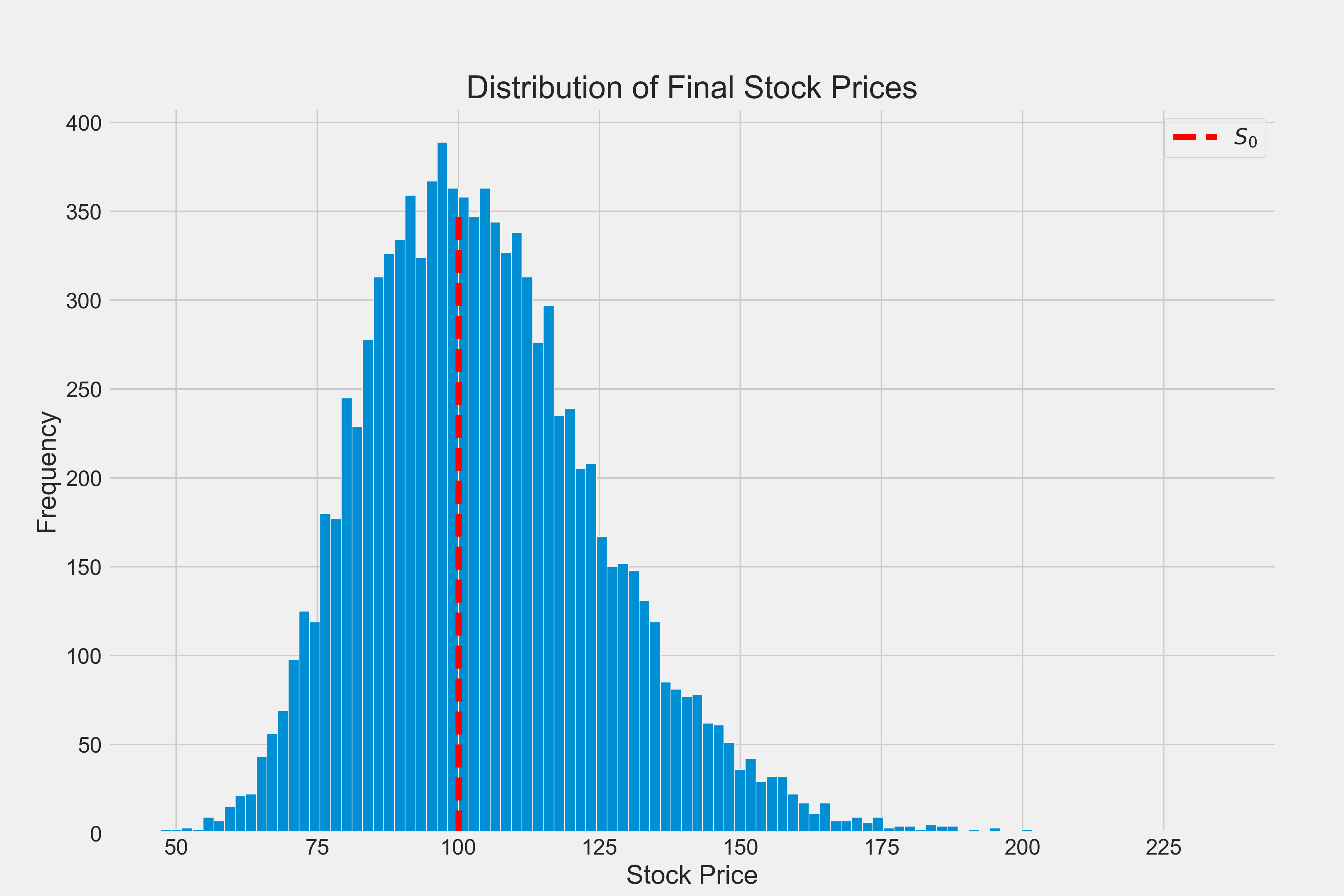
plt.figure(figsize=(10, 6))
plt.hist(paths[:, -1], bins=50)
plt.title("Distribution of Final Stock Prices")
plt.xlabel("Stock Price")
plt.ylabel("Frequency")
plt.show()
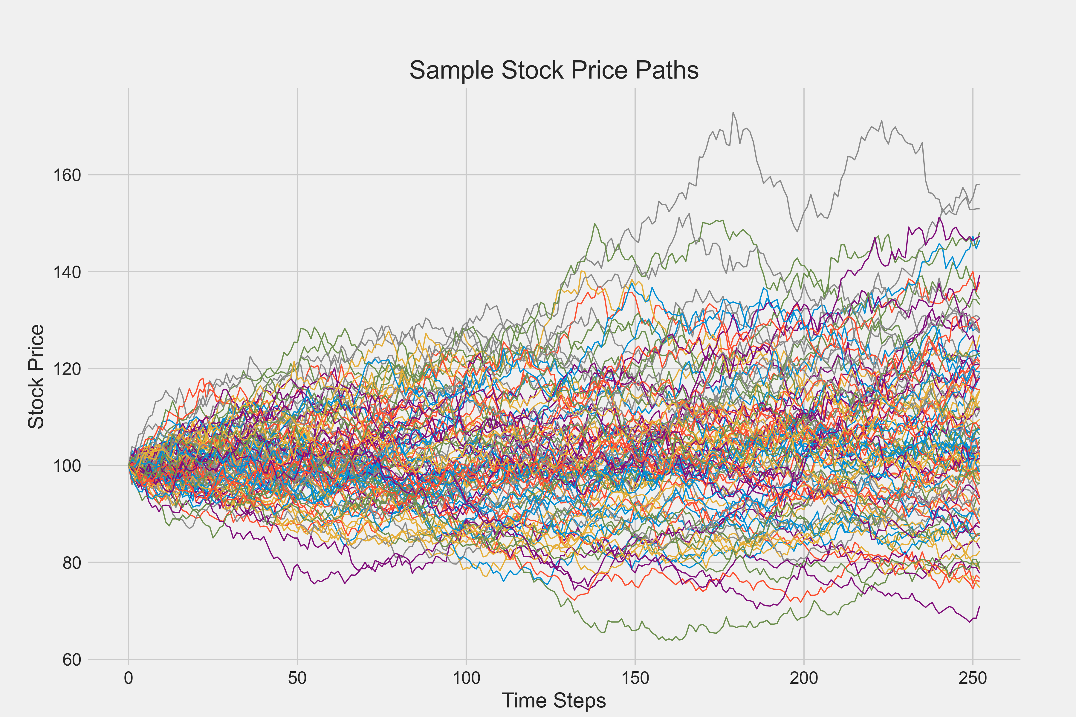
These visualizations show the range of possible stock price paths and the distribution of final stock prices, providing insight into the option’s potential outcomes.
6. Comparison with Analytical Solutions
To validate our Monte Carlo results, we can compare them with the Black-Scholes analytical solution:
from scipy.stats import norm

def black_scholes_call(S0, K, T, r, sigma):
    d1 = (np.log(S0 / K) + (r + 0.5 * sigma**2) * T) / (sigma * np.sqrt(T))
    d2 = d1 - sigma * np.sqrt(T)
    return S0 * norm.cdf(d1) - K * np.exp(-r * T) * norm.cdf(d2)

bs_price = black_scholes_call(S0, K, T, r, sigma)
print(f"Black-Scholes price: {bs_price:.3f}")
print(f"Monte Carlo price: {price:.3f}")
print(f"Difference: {abs(bs_price - price):.4f}")
The difference between the two methods gives us an idea of the Monte Carlo simulation’s accuracy.
Black-Scholes price: 11.270
Monte Carlo price: 11.445
Difference: 0.1744
7. Advanced Topics and Extensions
Monte Carlo simulation’s flexibility allows for various extensions:
- Variance Reduction Techniques: Methods like antithetic variates can improve accuracy without increasing computational cost.
- Exotic Options: Monte Carlo can price complex options like Asian or barrier options, which are challenging for analytical methods.
- Incorporating Dividends: We can easily modify the simulation to account for dividend payments.
- Stochastic Volatility: Models like Heston can be implemented to account for changing volatility.
8. Conclusion
Monte Carlo simulation offers a powerful and flexible approach to option pricing, addressing many limitations of analytical methods like the Black-Scholes model. While it can be computationally intensive, it handles complex scenarios and option structures with relative ease.
The method’s ability to incorporate various market dynamics, such as changing volatility or dividend payments, makes it invaluable in real-world financial modeling. As computational power continues to increase, Monte Carlo methods are likely to play an even more significant role in quantitative finance.
However, it’s important to remember that any model, including Monte Carlo simulation, is only as good as its underlying assumptions. Careful consideration of these assumptions and regular validation against market data remain crucial in applying these techniques effectively in practice.